NumPy - Logistic Distribution
什么是 Logistic Distribution?
Logistic Distribution 是一种连续概率分布,用于建模增长和 logistic regression。
它由两个参数定义:位置参数 μ(均值)和尺度参数 s。该分布类似于正态分布,但具有更重的尾部,这意味着它具有更高的极值概率。
示例:Logistic distribution 可以描述人口增长,其中增长率与现有数量和剩余增长量成正比。
Logistic distribution 的概率密度函数 (PDF) 定义为 −
f(x; μ, s) = (e-(x-μ)/s) / (s * (1 + e-(x-μ)/s)2)
其中,
- μ: 位置参数(均值)。
- s: 尺度参数(与标准差相关)。
- x: 随机变量的值。
- e: 欧拉数(约 2.71828)。
使用 NumPy 生成 Logistic Distributions
NumPy 提供了 numpy.random.logistic() 函数来从 logistic distribution 生成样本。您可以指定位置参数 μ、尺度参数 s 以及生成的样本大小。
示例
在本示例中,我们从位置参数 μ=0 和尺度参数 s=1 的 logistic distribution 生成 10 个随机样本 −
import numpy as np

# 从 μ=0 和 s=1 的 logistic distribution 生成 10 个随机样本
samples = np.random.logistic(loc=0, scale=1, size=10)
print("Random samples from logistic distribution:", samples)
以下是得到的结果 −
Random samples from logistic distribution: [-1.6473898   1.18698013 -0.24048488 -1.05235482  3.11858778 -1.40235809
  0.8399973  -1.46670621 -3.14359949 -0.80023521]
可视化 Logistic Distributions
可视化 logistic distributions 有助于更好地理解其特性。我们可以使用 Matplotlib 等库创建直方图来显示生成样本的分布。
示例
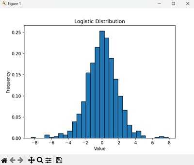
在以下示例中,我们首先从 μ=0 和 s=1 的 logistic distribution 生成 1000 个随机样本。然后创建直方图来可视化该分布 −
import numpy as np
import matplotlib.pyplot as plt

# 从 μ=0 和 s=1 的 logistic distribution 生成 1000 个随机样本
samples = np.random.logistic(loc=0, scale=1, size=1000)

# 创建直方图来可视化分布
plt.hist(samples, bins=30, edgecolor='black', density=True)
plt.title('Logistic Distribution')
plt.xlabel('Value')
plt.ylabel('Frequency')
plt.show()
直方图显示了 logistic distribution 中值的频率。条形表示每个可能结果的概率,形成 logistic distribution 的特征性 S 形 −
Logistic Distributions 的应用
Logistic distributions 在各个领域用于建模具有极值的数 据。这里有几个实际应用 −
- Machine Learning: 在 logistic regression 中建模二元结果。
- Economics: 建模增长以及收入和财富的分布。
- Statistics: 使用 logistic model 分析和预测结果。
生成累积 Logistic 分布
有时,我们对 logistic 分布的累积分布函数 (CDF) 感兴趣,它给出了在该区间内获得最多包括 x 个事件在内的概率。
NumPy 没有内置的 logistic 分布 CDF 函数,但我们可以使用循环和 SciPy 库中的 scipy.stats.logistic.cdf() 函数来计算它。
示例
以下是在 NumPy 中生成累积 logistic 分布的示例 −
import numpy as np
import matplotlib.pyplot as plt
from scipy.stats import logistic
# 定义位置和尺度参数
loc = 0
scale = 1
# 生成累积分布函数 (CDF) 值
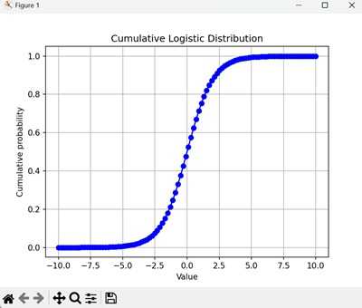
x = np.linspace(-10, 10, 100)
cdf = logistic.cdf(x, loc=loc, scale=scale)
# 绘制 CDF
plt.plot(x, cdf, marker='o', linestyle='-', color='b')
plt.title('Cumulative Logistic Distribution')
plt.xlabel('Value')
plt.ylabel('Cumulative probability')
plt.grid(True)
plt.show()
该图显示了在 logistic 试验中获得最多包括每个值在内的累积概率。CDF 是一条平滑曲线,随着值的增加而逐渐上升至 1 −
Logistic 分布的属性
Logistic 分布具有几个关键属性,例如 −
- 位置参数 (): 位置参数是分布的均值。
- 尺度参数 (s): 尺度参数与分布的标准差相关。
- 均值和方差: logistic 分布的均值为 ,方差为 (s22/3)。
- 偏度: 该分布围绕均值对称,其尾部比正态分布更厚。
使用 Logistic 分布进行假设检验
Logistic 分布常用于假设检验,特别是在二元结果的检验中。
一种常见的检验是 logistic regression,它用于基于一个或多个预测变量建模二元结果的概率。以下是使用 statsmodels 库的示例:
示例
在本示例中,我们对二元结果数据拟合一个 logistic regression 模型。摘要提供了模型的系数、标准误差和 p 值的信息 −
# Python version 3.11
import numpy as np
import statsmodels.api as sm

# 示例数据
X = np.array([0, 1, 2, 3, 4, 5])
y = np.array([0, 0, 0, 1, 1, 1])

# 为预测变量添加常数项
X = sm.add_constant(X)

# 拟合 logistic regression 模型
model = sm.Logit(y, X)
result = model.fit(method='lbfgs', maxiter=100, disp=0)

# 打印模型摘要
print(result.summary())
得到的输出如下所示 −
                           Logit Regression Results
==============================================================================
Dep. Variable:                      y   No. Observations:                    6
Model:                          Logit   Df Residuals:                        4
Method:                           MLE   Df Model:                            1
Date:                Wed, 20 Nov 2024   Pseudo R-squ.:                   1.000
Time:                        12:29:27   Log-Likelihood:            -5.7054e-05
converged:                       True   LL-Null:                       -4.1589
Covariance Type:            nonrobust   LLR p-value:                  0.003926
==============================================================================
                 coef    std err          z      P>|z|      [0.025      0.975]
------------------------------------------------------------------------------
const        -52.2706    668.240     -0.078      0.938   -1361.997    1257.456
x1            20.9332    265.301      0.079      0.937    -499.046     540.913
==============================================================================

Complete Separation: The results show that there iscomplete separation or perfect prediction.
In this case the Maximum Likelihood Estimator does not exist and the parameters
are not identified.
为可重复性设置种子
为了确保可重复性,您可以在生成 logistic 分布之前设置一个特定的种子。这确保了每次运行代码时生成相同的随机数序列。
示例
在本示例中,我们在从 logistic 分布生成随机样本之前将种子设置为 42。种子确保了每次运行代码时生成相同的样本序列 −
import numpy as np

# 为可重复性设置种子
np.random.seed(42)

# 生成 10 个来自 loc=0 和 scale=1 的 logistic 分布的随机样本
samples = np.random.logistic(loc=0, scale=1, size=10)
print("Random samples with seed 42:", samples)
以上代码的输出如下 −
Random samples with seed 42: [-0.51278827 2.95957976 1.00476265 0.39987857 -1.68815492 -1.68833811-2.78603295 1.86756387 0.41011316 0.88604138]