SciPy - Laplacian Filter

SciPy 中的 Laplacian Filter

Laplacian filter 是一种二阶导数滤波器，用于突出图像中强度急剧变化的区域，如边缘。它计算 x 和 y 方向二阶导数的总和，即 Laplacian。

对于 2D 图像 I(x,y)，数学上 Laplacian 表示如下 −

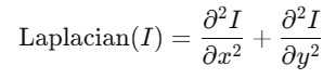
此操作捕获强度急剧变化的区域。当我们想使用 scipy 库实现 Laplacian filter 时，可以使用函数 scipy.ndimage.laplace()。

语法

以下是 scipy.ndimage.laplace() 函数的语法 −

scipy.ndimage.laplace(input, output=None, mode='reflect', cval=0.0)

以下是函数 scipy.ndimage.laplace() 的参数 −

• input: 输入数组，即应用滤波器的图像。
• output(optional): 用于存储结果的数组。如果未提供，则创建一个新数组。
• mode: 该参数定义输入数组在其边界处如何扩展。模式可以是 'reflect'、'constant'、'nearest'、'mirror' 和 'wrap'。
• cval: 如果 mode='constant'，则用于填充边缘以外的值。默认值为 0.0。

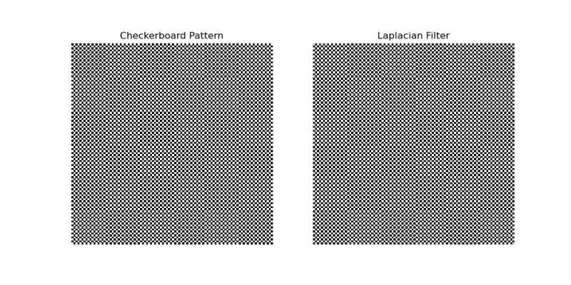
在合成图像上应用基本的 Laplacian Filter

以下示例展示了如何使用 scipy.ndimage.laplace() 函数在合成图像上应用基本的 Laplacian Filter −

import numpy as np
import matplotlib.pyplot as plt
from scipy import ndimage

# 创建合成棋盘图案
x = np.indices((100, 100)).sum(axis=0) % 2
image = x.astype(float)

# 应用 Laplacian filter
laplacian = ndimage.laplace(image)

# 绘图
plt.figure(figsize=(10, 5))
plt.subplot(1, 2, 1)
plt.title("Checkerboard Pattern")
plt.imshow(image, cmap='gray')
plt.axis('off')

plt.subplot(1, 2, 2)
plt.title("Laplacian Filter")
plt.imshow(laplacian, cmap='gray')
plt.axis('off')
plt.show()

以下是应用在给定图像上的基本 Laplacian filter 的输出 −

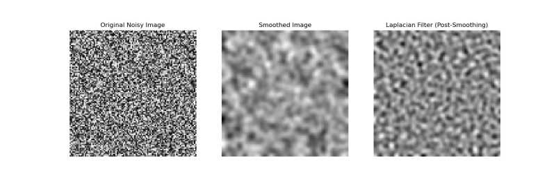
带预平滑的 Laplacian Filter

带预平滑的 Laplacian filter 是一种图像处理技术，在应用 Laplacian filter 之前先使用 Gaussian filter 来减少噪声。这种组合在边缘检测中很有效，同时能最小化噪声伪影。以下示例在噪声图像上先应用 Gaussian filter，然后再应用 Laplacian filter −

import numpy as np
from scipy import ndimage
import matplotlib.pyplot as plt

# 创建噪声图像
np.random.seed(42)
image = np.random.random((100, 100))

# 在 Laplacian filter 之前应用 Gaussian 平滑
smoothed = ndimage.gaussian_filter(image, sigma=2)
laplacian = ndimage.laplace(smoothed)

# 绘图
plt.figure(figsize=(15, 5))
plt.subplot(1, 3, 1)
plt.title("Original Noisy Image")
plt.imshow(image, cmap='gray')
plt.axis('off')

plt.subplot(1, 3, 2)
plt.title("Smoothed Image")
plt.imshow(smoothed, cmap='gray')
plt.axis('off')

plt.subplot(1, 3, 3)
plt.title("Laplacian Filter (Post-Smoothing)")
plt.imshow(laplacian, cmap='gray')
plt.axis('off')
plt.show()

以下是应用带预平滑的 Laplace Filter 的输出 −

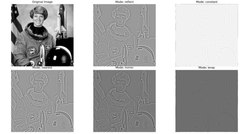
拉普拉斯滤波器与边界模式

在拉普拉斯滤波器和高斯平滑中，边界模式控制卷积过程中图像边缘的处理方式。这一点很重要，因为滤波器会操作超出原始图像边界的位置。在这个示例中，我们将 mode 参数传递给 scipy.ndimage.laplace() 函数 −

import numpy as np
import matplotlib.pyplot as plt
from scipy import ndimage
from skimage import data, color

# 第1步：加载图像
image = color.rgb2gray(data.astronaut())  # 转换为灰度图

# 第2步：使用高斯滤波器预平滑
sigma = 2
smoothed_image = ndimage.gaussian_filter(image, sigma=sigma)

# 第3步：使用不同模式应用拉普拉斯滤波器
modes = ['reflect', 'constant', 'nearest', 'mirror', 'wrap']
results = {}

for mode in modes:
    laplacian = ndimage.laplace(smoothed_image, mode=mode, cval=0)  # 'constant' 模式使用 cval=0
    results[mode] = laplacian

# 第4步：可视化结果
plt.figure(figsize=(15, 10))
plt.subplot(2, 3, 1)
plt.title("原始图像")
plt.imshow(image, cmap='gray')
plt.axis('off')

for i, mode in enumerate(modes, start=2):
    plt.subplot(2, 3, i)
    plt.title(f"模式: {mode}")
    plt.imshow(results[mode], cmap='gray')
    plt.axis('off')

plt.tight_layout()
plt.show()

以下是应用预平滑后的拉普拉斯滤波器的输出结果 −